Housing Cycle Analysis
US real estate cycle tracked through cascading leading, confirming, and lagging indicators.
Last Update: --
Housing Cycle Score
Signal Cascade
Values = Strength (0-100). Above 65 = expansion, below 35 = contraction. Peak = last date above 65.
Key Indicators
Federal Reserve Economic Data (FRED)
International Housing Cycles
Housing cycle strength based on BIS real and nominal property price indices (2010=100). Select a country to see its cycle history.
Understanding the Housing Cycle
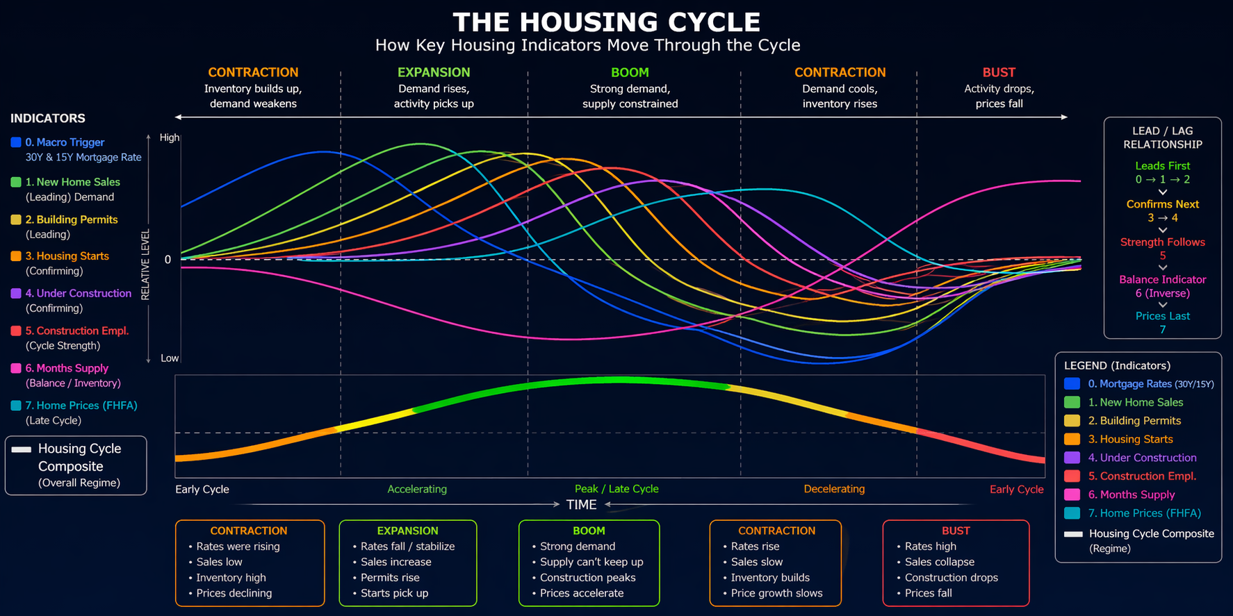
The Signal Cascade
Housing markets follow a predictable chronological sequence. Each indicator peaks at a different point in the cycle, creating a cascade from leading to lagging signals. Understanding this sequence allows early detection of cycle turns.
Individual Indicators
0. Mortgage Rates (Macro Trigger)
The 30-Year and 15-Year Fixed Mortgage Rates are the exogenous trigger that starts and ends housing cycles. When rates fall, borrowing becomes cheaper and demand explodes. When rates rise, affordability drops and demand collapses. This is the earliest signal — it leads the entire cascade by 6-18 months. Inverted in the composite: lower rates = higher score.
1. New Home Sales (Demand — Leading)
The first endogenous response to rate changes. Buyers enter or leave the market immediately. A sustained rise in new home sales signals early-cycle recovery; a sustained decline is the first warning of a downturn. Data from the US Census Bureau, monthly, since 1963.
2. Building Permits (Supply Intent — Leading)
Developers react to rising demand by applying for building permits. This is a pure forward-looking indicator — it reflects expectations, not reality. Permits typically peak 3-6 months after sales. A sharp drop in permits signals developers expect demand to weaken. Monthly, since 1960.
3. Housing Starts (Supply Execution — Confirming)
When permits are approved, construction begins. Housing Starts confirm that the cycle is real — developers are committing capital. Starts lag permits by 1-3 months. A divergence (permits rising but starts flat) suggests developers are cautious despite demand. Monthly, since 1959.
4. Units Under Construction (Pipeline — Confirming)
The construction pipeline measures ongoing activity. It rises slowly as starts accumulate and falls slowly as projects complete. A rising pipeline means the boom is stable; a falling pipeline means the cycle is weakening. This is a mid-cycle indicator with significant inertia. Monthly, since 1968.
5. Months Supply (Balance — Transition)
The ratio of homes available for sale to the monthly sales rate. Low supply (below 4 months) means a tight market with upward price pressure. High supply (above 7 months) means an oversupplied market with downward pressure. Often the turning point indicator — when supply starts rising from lows, the cycle may be peaking. Inverted: lower supply = higher score. Monthly, since 1963.
6. Residential Construction Employment (Cycle Strength — Lagging)
The labor market responds last. Companies hire only when the boom is established and fire only when the downturn is undeniable. Employment data from the BLS confirms the cycle phase but doesn't predict turns. Monthly, since 1985.
7. Home Prices — FHFA HPI (Late Cycle — Lagging)
Home prices react last in the cascade. They continue rising even after sales peak (sticky prices, pending contracts) and continue falling after the bottom in sales (foreclosure overhang). The FHFA House Price Index is used instead of Case-Shiller because it's Public Domain (redistributable), while Case-Shiller requires S&P licensing. Quarterly, since 1975.
Composite Score & Strength Indicator
Each raw indicator is transformed into a Strength Indicator (0-100 oscillator) using: EMA(10) / SMA(25) ratio, min-max normalized over a 260-period rolling window, then smoothed with an Ehlers 2-pole Super Smoother filter for minimal-lag noise reduction.
The composite Housing Cycle Score is a weighted average of tier strengths:
- Tier 0 — Macro Trigger (15%): Mortgage Rates (inverted)
- Tier 1 — Leading (25%): New Home Sales + Building Permits
- Tier 2 — Confirming (25%): Housing Starts + Under Construction
- Tier 3 — Balance (20%): Months Supply (inverted)
- Tier 4 — Lagging (15%): Employment + Home Prices + Median Price
Regime Classification
- Boom (Score >= 80): All indicators aligned bullish — strong demand, tight supply, rising prices
- Expansion (Score >= 65): Broad improvement — leading indicators rising, construction accelerating
- Neutral (Score 35-65): Mixed signals — transition phase, leading and lagging may diverge
- Contraction (Score <= 35): Broad deterioration — demand falling, permits declining
- Bust (Score <= 20): All indicators aligned bearish — high rates, collapsing sales, rising inventory
Data Sources: FRED (US Census Bureau, FHFA, Freddie Mac, BLS — Public Domain with citation). International data from BIS (61 countries) and Eurostat (37 EU countries, CC-BY 4.0).